Suppose I offer you a bet. Flip a coin, heads you lose your entire bet, tails you win it back plus one and a half times, so a ten dollar bet becomes $25. And furthermore I’ll let you keep making this bet as many times as you like over the next hour, say.
This is a fantastic bet. For a $10 wager the expected payoff is (0.5 * $0) + (0.5 * $25) = $12.50, or a 25% expected return on invested capital, in the amount of time it takes to flip a coin. Stock markets don’t offer half those expected profits over a year’s time. You should keep making this bet for as long as I will let you. But how much money should you be betting? The more you bet the more you stand to gain, at highly favorable odds, but if your answer is “all the money I have to my name” then you’re doing it wrong.
Why? Because my bet is only valuable to you for as long as you have money to keep making it. But if you bet too much, you will eventually go bust. The world’s best bet can destroy you if you don’t manage your bankroll prudently. This may sound obvious, but in one experiment that offered participants the chance to bet real money on a similarly favorable series of coin flips, 28% lost their entire bankroll while only 21% managed to win the maximum allowable amount. Only a few of the participants followed the optimal betting strategy, a finding made all the more terrifying by the fact that the sample consisted of students in economics and professional financial analysts. That optimal strategy, known as the Kelly Criterion, is an underappreciated gem of applied mathematics. Brought into being by a Texan gunslinger, mastered by the world’s first card counter, and used today by some of the most successful investors alive, the Kelly Criterion can tell us what was behind the biggest blowups in finance, why levered ETFs are generally a bad idea, and how aggressive investors can maximize their wealth without risking ruin.
Some Very Interesting Geeks
John Kelly, Jr. was a WWII air force pilot and oilman before joining the famous research and development company Bell Labs at the age of 30. Among the scientists and engineers at its New Jersey campus, Kelly stood out due to his Texan drawl, chain-smoking habit, and penchant for firearms, firing homemade bullets at parties to impress guests, as well for his sharp intelligence; many people at Bell Labs at the time said he was the smartest person there after Claude Shannon. This was no faint praise, as Shannon was one of the key contributors to the development of the digital computer, and the father of information theory.
Information Theory is, as Shannon’s original 1948 paper called it, “A Mathematical Theory of Communication.” It concerns what are the theoretical limits to signal processing and data compression. Shannon originally conceived of the problem by considering how, when a message is being transmitted over a channel that contains random noise, the message can be received and decoded with minimal probability of error, a matter of great practical concern to Bell Labs’ AT&T overlords. Shannon’s insights contributed to our understanding of topics like uncertainty, entropy, and even led to the concept of the “bit” of information. Information theory has found applications in fields as far ranging as thermal physics, molecular biology, and artificial intelligence. But its first extension was to gambling.

Claude Shannon, with his famous “I’m a genius” look
Kelly had heard about a gambling scam on the news in which the outcome of a quiz show was being telephoned to confederates and bet upon before the show aired. Thinking about the strategy such cheaters should follow, Kelly realized that Shannon’s equations were applicable. Shannon urged Kelly to publish his findings, and he did so in an article titled “A New Interpretation of Information Rate” (he had originally chosen the title “Information Theory and Gambling,” but his superiors at AT&T, who did a lot of business with bookies they didn’t want to draw undue attention towards, opted for a more opaque name).
In the paper, Kelly considered the case of a horse race bettor with a “private wire” that gives him advance word of the race’s outcome. Though it seems intuitive that such a gambler should bet all he can on such a rigged game, Kelly realized that can’t be correct. Just as Shannon deduced that a communication channel always contains some amount of random noise that reduces the information content of the message transmitted, Kelly reasoned that there was always some chance that our gambler could receive a bum tip, or that there would be some other error – or noise – in the system, and the first time there was the gambler would surely lose everything if he were betting everything. On the other hand, of course, if the gambler were too conservative and bet too little he would give up a tremendous amount of profit. There had to be an optimal amount of money to put at stake.
This Goldilocks bet is given by the following formula, what has since come to be called the Kelly Criterion:
f = bp – q / b
Where f is the fraction of her bankroll a gambler should bet, b is the betting odds or payout in the case of a win, p is the probability of winning and q is the probability of losing.
Let’s reconsider the coin flip I imagined offering up top. Far from betting everything on heads or tails, the Kelly Criterion says the optimal bet size is (2.5 * 50% – 50%) / 2.5 = 30% of your bankroll. While we can prove this maximizes the growth rate of your bankroll with some calculus, a Monte Carlo simulation illustrates the point a little more intuitively. Below I simulate the hypothetical growth of four different gamblers’ wealth each betting a different fraction of their bankroll on my coin flipping game over 100 flips. In each case I used a random number generator to simulate a coin flip and ran 1000 trials for each gambler, then plotted the median wealth after each flip.
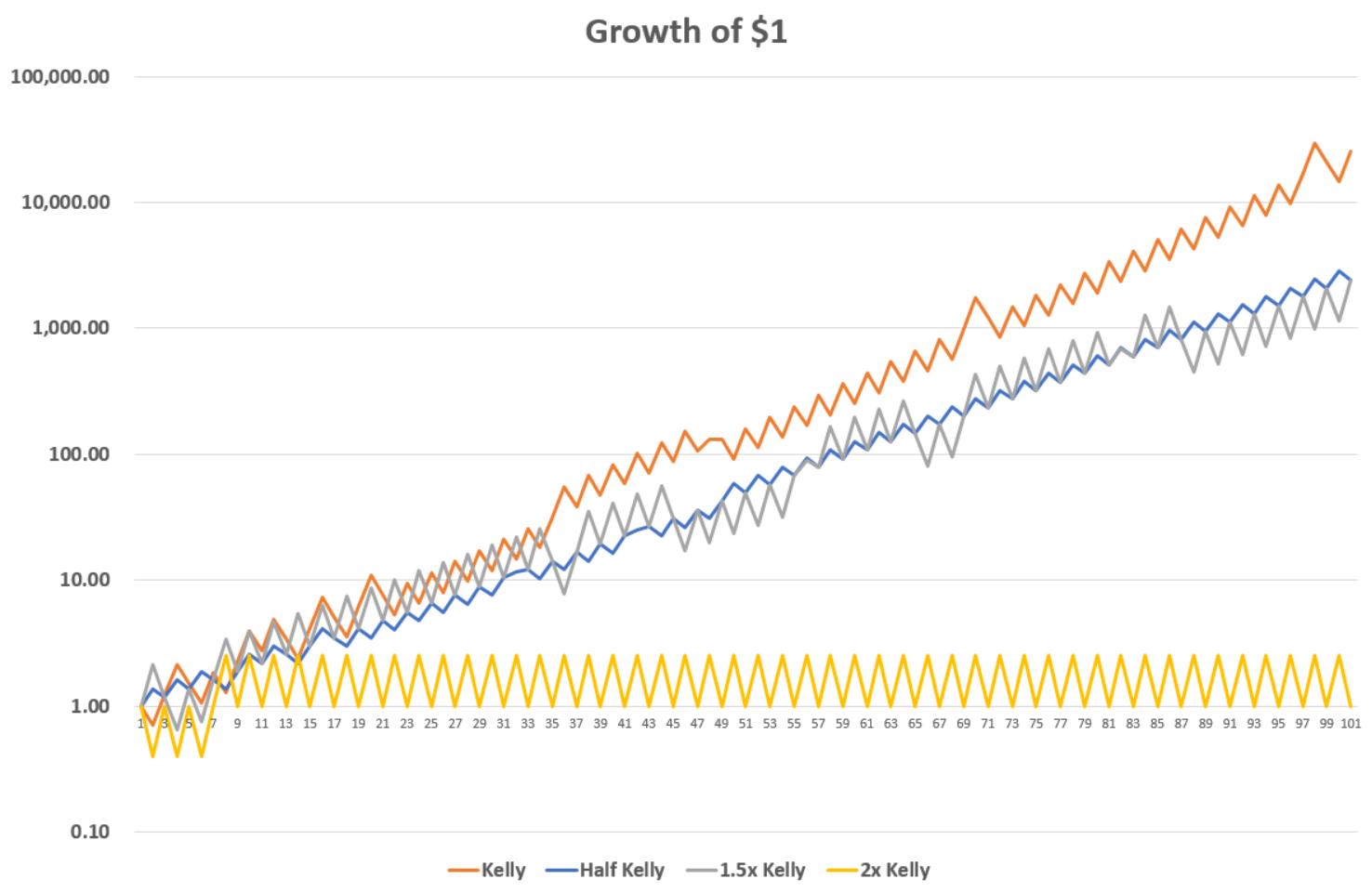
The Kelly bettor bets the “correct” 30% proportion of his bankroll each flip. “Half Kelly” underbets, risking 15% each flip; “1.5x Kelly” overbets with 45% stakes and “2x Kelly” is wilder still, betting 60%. As you can see, though the more aggressive bettors do spend some brief points in the lead within the first few flips (an artifact of the random element that goes away in the limit), the Kelly bettor eventually pulls decisively into the lead, ending with a terminal wealth of about $25,515. Betting less than 30% doesn’t allow a gambler to compound his wealth nearly as fast, but on the other hand betting too much means every losing toss sets the gambler too far back, also detracting from growth, and so the half Kelly and 1.5x Kelly bettors substantially underperform, ending up with the same terminal wealth of $2,432, as the math would have it, though the 1.5x Kelly bettor experiences much wider swings in wealth flip-to-flip. The 2x Kelly bettor loses so much on each bad flip that he is never able to get off the ground, and ends up exactly where he started. Betting more than 60% would result in erosion and ultimate depletion of wealth.
John Kelly died young and supposedly never put his own formula to use. That would have to wait for another associate of Claude Shannon’s… Shannon moved to MIT in 1956 and that same year was asked to review a paper from a young new adjunct mathematics professor named Edward Thorp before it could be submitted for journal publication. In his paper, Thorp demonstrated the first mathematical proof that the game of blackjack could be played so as to move the odds in favor of the player instead of the dealer, something most mathematicians had long assumed was impossible. Thorp showed that by keeping track of the cards as they are dealt and betting more when the deck contains relatively more favorable cards and less when contrariwise, a player could obtain a substantial edge over the dealer. Shannon was fascinated and immediately became a close friend and collaborator with Thorp. He also recommended that Thorp look into the work of John Kelly. Armed with his system of card counting and the Kelly criterion for optimal bet sizing, Ed Thorp spent the next handful of years winning a small fortune in Nevada casinos and published the bestselling book Beat the Dealer about his strategy, much to the chagrin of casinos everywhere. (Thorp and Shannon went into business together for a while as well, together building the world’s first wearable computer, which they used to predict the outcome of roulette games.)
Thorp eventually got tired of taking casinos’ money and set his sights on a more ambitious target: Wall Street. Starting with managing some friends’ money in his spare time, he eventually cofounded a hedge fund called Princeton Newport Partners. At PNP, Thorp ran various arbitrage strategies while keeping a fastidious focus on risk, consistent with his mathematical background in bet-sizing. The results were perhaps the greatest risk-adjusted returns any hedge fund had ever delivered before or since. Between 1969 and 1988 Princeton Newport had a compound annualized return of 19.1% vs. the S&P 500’s 10.2%. What’s more, over its two decades in operation, PNP only lost money in three months, and its returns were completely uncorrelated with those of the stock market or any other risky asset. All the while, Thorp continued to publish mathematical research, including elaborations on the Kelly Criterion and its extensions to other situations like stock investing.
If you want to learn how to apply this methodology to your portfolio schedule a call with us HERE.
How Much Leverage is Too Much?
Because of increased competition, it’s unlikely that any investor will ever again match Thorp’s remarkable performance record, but the formulas of Thorp and Kelly can still be useful to investors everywhere in managing risk and return. In particular, the Kelly criterion can be adapted to the continuously varying mathematics of the market to tell us how much leverage to use. Assuming the existence of some asset (or portfolio of assets) with normally distributed returns and a risk-free asset (typically assumed to be short-term government bonds) that we can have positive or negative allocations in (a negative position in the risk-free asset means we’re borrowing money means we’re using leverage), then the Kelly Criterion of asset a takes on the following form (sometimes referred to as the Kelly Capital Growth Investment Criterion):
f = Expected Return_a – Risk Free Rate / Volatility_a^2
That is, the fraction f that we should allocate to the asset in order to maximize returns is equal to the return the asset is expected to deliver in excess of the risk free rate, divided by the square of the asset’s volatility as measured by its standard deviation of returns (this is simply the asset’s variance). Values of f greater than 1 indicate allocations of more than 100%, i.e. the use of leverage.
In my last post I railed against levered ETFs, investment products that have collectively cost investors billions of dollars. Despite this we at RHS Financial have had positive things to say about leverage before, and leverage is an integral part of the investment strategies we employ. Armed with the Kelly capital growth investment criterion, we can now square that circle and distinguish between good and bad uses of leverage. Let’s start by considering SPY, the world’s first ETF, indexed to the S&P 500. SPY gave individual investors the ability to trade virtually the entire stock market in continuous, real time, which means it also gave individual investors the ability to adjust their leverage to the market in real time as well, so it will serve as our baseline. $1 invested in SPY since its inception in 1993 would have grown to $8.67 by the end of May 2017 with reinvested dividends. That’s a 9.28% annualized return. Not bad.

Comparing against the rate on 3 month treasury bills over this period, SPY had an average excess daily return of 0.032% and a daily return volatility of 1.166%. Plugging in the numbers, that means the Kelly leverage ratio was 2.37. That is, assuming a constant leverage ratio, a Kelly investor would have maximized her return over this period by rebalancing each day to hold 237% of her capital in SPY, financing her excess over 100% by borrowing at the rate of T-bills1Technically the Kelly capital growth investment formula assumes normally distributed returns, and returns on financial assets are notoriously non-normal. Accounting for the higher moments of the distribution will generally result in lower optimal levels of leverage, but for moderate leverage levels applied to broadly diversified portfolios, the differences are generally trivial. In this particular case the true optimal ex-post leverage ratio is 2.36, a 1% difference. I will ignore the effects of higher moments throughout the rest of the post.. Doing so would have looked like this:
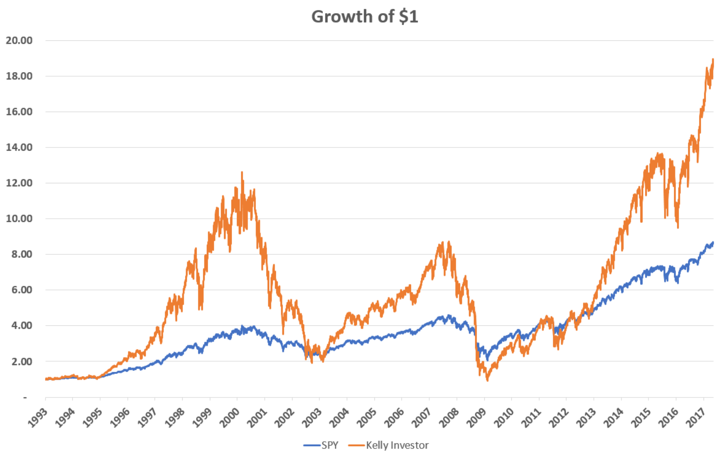
Wheeeeee! Investing with 237% leverage in SPY would have maximized returns over this 24 year period, but it would have been a wild ride. The Kelly investor would have completely lost their lead to the unlevered investor twice over the years following both the dot-com bust and the 2008 financial crisis before finally finishing in May 2017 with a terminal wealth of $18.88, an annualized return of 12.84%.
A few caveats: this “backtest” is totally cheating. An investor in 1993 would obviously have had no way of knowing what the average daily return and volatility on the S&P 500 would be over the next 24 years. In real life we can only estimate these parameters with great uncertainty. Not to mention I have not accounted for transaction costs here, which could be significant with daily rebalancing. Still, this illustrates my point about the Kelly formula and optimal leverage, which we can throw into greater relief by considering other leverage ratios over the same period.
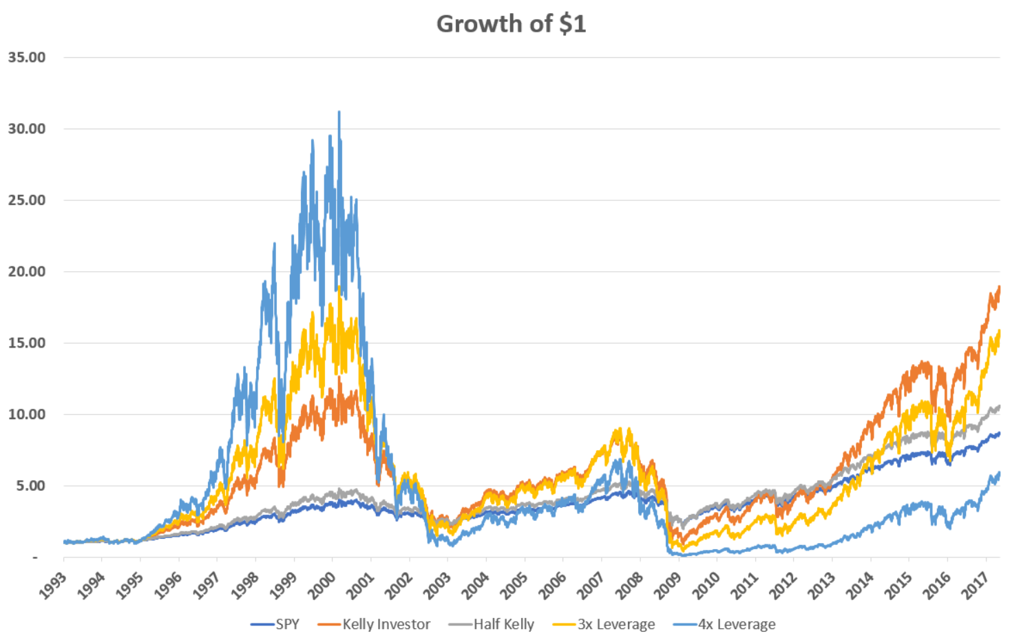 In the graph above I add a more conservative “Half Kelly” investor that invests only 119% of his capital in SPY each day, as well as 3x and 4x levered counterparts. Not surprisingly, the half Kelly investor does better than the unlevered SPY (but with more risk) but worse than the full Kelly investor (but with less risk). Less intuitively, using more than 2.37x leverage does not improve returns. The 3x levered investor ends with $15.83 (a 12.02% annualized return) and the 4x levered investor does even worse than SPY itself, ending with only $5.89 (a 7.56% annualized return). Though not pictured here, using 5x leverage would have lost money in absolute terms, turning a dollar into 89 cents over 24 years.
From this we start to see the problem with levered ETFs as they are currently constructed: they generally use too much leverage applied to too volatile of assets. Even with the plain vanilla S&P 500 3x leverage is too much. And after accounting for the hefty transactions costs and management fees these ETFs charge, even 2x might be suboptimal (especially if you believe returns will be lower in the future than they have in recent decades). And the S&P 500 is one of the most conservative targets for these products. Take a look at the websites of levered ETF providers and you will see ways to make levered bets on particular industries like biotech or the energy sector, or on commodities like oil and gold, or for more esoteric instruments yet, almost all of which are more volatile than a broadly diversified index like the S&P 500, and thus supporting much lower Kelly leverage ratios, probably less than 2x.
Let us instead go in the opposite direction and consider levering up less volatile assets. As I wrote about in an earlier post on leverage, when looking at the stock market, those stocks that have had the least volatile returns in recent periods tend to perform about just as well as the overall market, but with (obviously) less volatility, implying they support a higher Kelly leverage ratio. As our proxy for low volatility stocks, let’s look at the S&P 500 Low Volatility Index, an index that tracks the 100 stocks in the S&P 500 with the least realized volatility over the trailing year. A popular ETF based on this index, SPLV, launched in 2011, but I want to look at the same period since 1993 so I will use the index data itself (with the additional caveat that indexes are not directly investable and so this backtest will be even less realistic than the last one). Below I plot the returns of SPY, the SPLV index, and an investor applying Kelly leverage to SPLV.
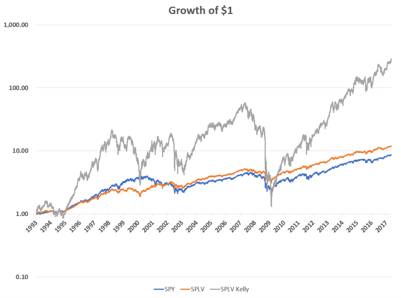
Over the same 1993-2017 period low volatility stocks actually outperformed the S&P 500, 10.77% vs. 9.28%, and had a much lower daily volatility of 0.84%, only about two thirds that of the S&P 500. That translates to a Kelly leverage ratio of 4.85, more than double what we had above for SPY. The Kelly investor thus goes from a terminal wealth of $18.88 with SPY to $291.99 with SPLV, a phenomenal 26.28% annualized return. Again, the Kelly investor would have had to endure incredible amounts of volatility to get there, especially during the financial crisis, and again this backtest is unrealistic for several reasons, but we see the principle at work behind rational levered investing. The Kelly criterion sets an upper bound for an investor dividing the realms of “aggressive” and “crazy.” By focusing more on low volatility investments, the investor can push that dividing line up further still.
Now, the best way to reduce portfolio volatility is through diversification, especially by including assets with low or negative correlations with each other. From the perspective of an equity investor, the most diversifying asset class is government bonds, which tend to rally during recessions when investors rush to safety and lag during stock bull markets. Thus the zigs of government bonds largely offset the zags of the stock market, and so including them in a portfolio can greatly reduce overall volatility.
Below I plot the returns of SPY, as well as a portfolio that’s 50/50 SPLV and long-term government bonds (proxied by the ETF TLT since its inception in 2002, and by the Vanguard mutual fund VUSTX before then) and a Kelly investor in the 50/50 portfolio.
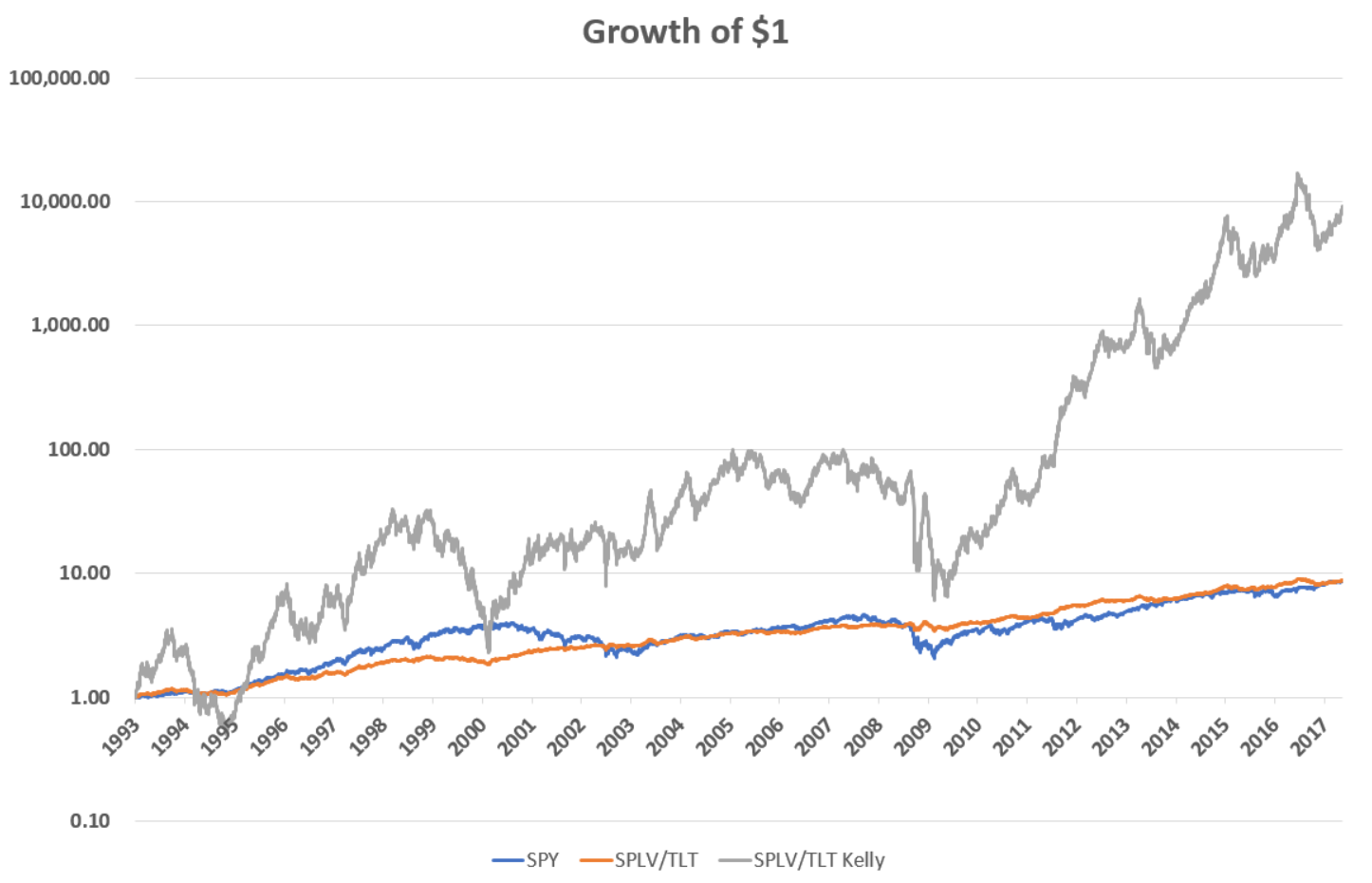
We have now entered the stratosphere. The annualized total return of the combined SPLV/TLT portfolio was 9.36%, almost exactly the same as SPY. It achieved this, however, with substantially less risk, its growth path almost looking like a straight line on the graph above. In fact, its daily volatility was 0.51%, less than half of SPY’s. This means the Kelly leverage ratio is now a whopping 10.38 and our Kelly investor turns their dollar into $9,067 by 2017. This represents a return of 45.44%, the sort of performance one normally associates with Ponzi schemes, only we did it with math. Well, math plus some completely unrealistic assumptions, an additional one this time around being the fact that no broker will ever let you use this much leverage on these securities. And again, even if this were realistic, I wouldn’t recommend this portfolio to anybody except maybe those with chronically low blood pressure. The annualized volatility of the Kelly portfolio is an eye-popping 84% (over 4 times that of SPY) and the Kelly investor would have experienced 3 episodes of 80%+ drawdowns. The Kelly criterion merely tells us the maximum amount of risk an investor can take to increase return, not whether that level is desirable or not. Fortunately, there’s a great deal of space between the orange line and the grey line above for an investor to strive to find the right balance for themselves.
Okay, now let’s try to take an important step towards realism. As I mentioned, all these simulations above suffer from look-ahead bias, that is, I created them using data from over my sample period that an investor couldn’t possibly have had access to at the time (not without a time machine, anyway). In reality, investors have to try to estimate what future returns and risks will be using only information that is available at the present moment. This is a task fraught with uncertainty, but not necessarily futile. As I’ve talked about before, future stock market returns can be estimated, albeit with a great deal of noise, using the earnings yield; that is, the aggregate earnings of stocks (usually averaged over a period of ten years) divided by the current price level of the market. The expected return on bonds can be more easily and accurately estimated by simply looking at the current yield to maturity of the bond market. There is also a vast academic literature on forecasting volatility, with a cornucopia of elaborate statistical models developed by Ph.D. mathematicians and deployed by quantitative hedge funds. But it turns out that simply assuming the volatility the market has experienced in the recent past will continue into the near future actually does a pretty good job in formulating forward-looking risk estimates. Combining all these estimates, we can create a simple model of how a Kelly investor should have traded in real time over the course of our sample period.
In the graph below, I plot the performance of SPY against two portfolios that allocate to a 50/50 SPLV/TLT portfolio using different real-time, forward looking estimates. One is a full Kelly investor trying to maximize returns regardless of risk. For each day over the sample period I estimate the expected returns on stocks and long-term government bonds based on their yields as well as the expected volatility of the portfolio to arrive at the day’s Kelly leverage ratio2Specifically, I calculate the expected return on stocks each day as the sum of the smoothed earnings yield (i.e. the inverse of the CAPE ratio for latest available data) and expected inflation, as measured by the latest available figure from the University of Michigan Survey of Consumers. I calculate the expected return on long-term government bonds as the latest available yield on the 20 year treasury bond. I assume expected volatility is equal the trailing 60 day realized volatility.. Thus the leverage increases (decreases) when expected returns are higher (lower) and leverage decreases (increases) when recent volatility is higher (lower). The other investor follows a perhaps more realistic, aggressive-but-not-maximally-aggressive strategy of targeting an annualized volatility level of 18%, which is approximately what the long-term volatility of the US stock market has been, both before and during our sample period, and is well within the bounds of the Kelly criterion. Due to data availability I begin at the start of 1994.
 Using real-time data, the full Kelly investor actually ends up with $16,719 at the end of the period (a 51.53% annualized return), better than the pseudo-clairvoyant Kelly investor in the previous chart. This is because by estimating volatility in real-time, the forward-looking Kelly investor is able to mitigate some of the worst drawdowns that the constant-leverage investor dealt with. This time the Kelly investor “only” deals with a couple ~70% drawdowns. Still, the performance is rather erratic, and the vast majority of it comes in the years following the financial crisis. High-risk-high-reward seeking investors must be patient! In contrast, by targeting a stock-market level of risk, the 18% volatility target investor outperforms SPY relatively consistently (by which I mean, periods of underperformance only last a few years at a time, a stretch most investors seem to find intolerable). He ends up with $63.51, or a 19.41% annualized return, more than double that of SPY. Though in reality transactions costs would have created a significant drag, and future returns are likely to be less than the ones seen here, an investor could also improve upon these simplistic models by incorporating additional asset classes and shifting allocations between them dynamically based on forward-looking risk and return estimates, at least in principle.
And thus we see how the Kelly criterion can tell us how much leverage is too much and how aggressive investors can seek to maximize their returns without losing their shirts. Next time we will continue pursuing this thread and ask, how can we profit by betting against those who bet too much?
Disclosures: This post is solely for informational purposes. Past performance is no guarantee of future returns. Investing involves risk and possible loss of principal capital. No advice may be rendered by RHS Financial, LLC unless a client service agreement is in place. Please contact us at your earliest convenience with any questions regarding the content of this post. For actual results that are compared to an index, all material facts relevant to the comparison are disclosed herein and reflect the deduction of advisory fees, brokerage and other commissions and any other expenses paid by RHS Financial, LLC’s clients. An index is a hypothetical portfolio of securities representing a particular market or a segment of it used as indicator of the change in the securities market. Indexes are unmanaged, do not incur fees and expenses and cannot be invested in directly.


